Source: Tektronix
Debugging embedded systems often involves looking for clues that are hard to discover just by looking at one domain at a time. The ability to look at time and frequency domains simultaneously can offer important insights.
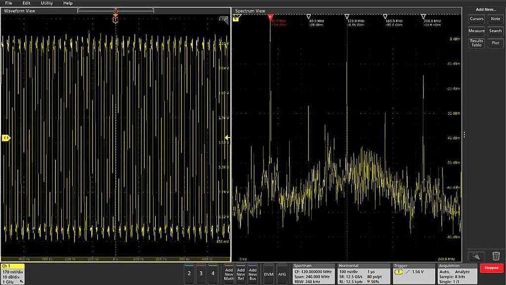
FIGURE 1. Spectrum View enables simultaneous analog and spectrum views with independent controls in each domain.
Debugging embedded systems often involves looking for clues that are hard to discover just by looking at one domain at a time. The ability to look at time and frequency domains simultaneously can offer important insights. Mixed domain analysis is especially useful for answering questions such as:
• What’s going on with my power rail voltage when I’m transmitting wireless data?
• Where are the emissions coming from every time I access memory?
• How long does it take for my PLL to stabilize after power-on?
Mixed domain analysis can help answer questions like these by providing views of time domain waveforms and frequency domain spectra in a synchronized view. Up until recently, the Tektronix MDO4000C mixed domain oscilloscope has been the only oscilloscope to offer synchronized time and frequency domain analysis with independent control over waveform and spectrum views.
To address this need, the 4, 5 and 6 Series MSO mixed signal oscilloscopes offer an analysis tool called Spectrum View. It is an option in the 4 Series MSO and a standard feature in the 5 and 6 Series MSOs. It delivers several key capabilities:
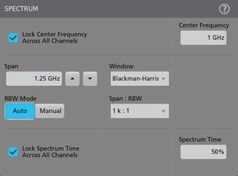
• Enables the use of familiar spectrum analysis controls (Center Frequency, Span and RBW)
• Allows optimization of both time domain and frequency domain displays independently
• Enables a signal to be viewed in both a waveform view and a spectrum view without splitting the signal into different inputs
• Enables accurate correlation of time domain events and frequency domain measurements (and vice versa)
• Significantly improves achievable frequency resolution in the frequency domain
• Improves the update rate of the spectrum display
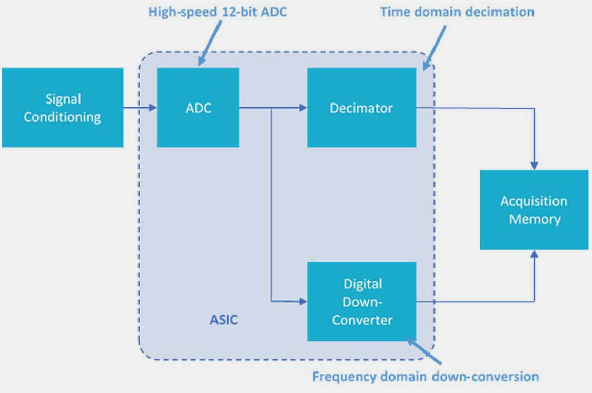 FIGURE 2. Digital down converters implemented on a custom ASIC enable simultaneous waveform and spectrum views with independent controls FIGURE 2. Digital down converters implemented on a custom ASIC enable simultaneous waveform and spectrum views with independent controls |
A new architecture
Spectrum View uses patented hardware built into the instruments. To understand how it works, it is important to note that digital oscilloscopes generally run their analog-to-digital converters (ADC) at the maximum sample rate. The stream of ADC samples is then sent to a decimator that keeps every Nth sample. At the fastest sweep speeds, all samples are kept. At slower sweep speeds, it’s assumed the user is looking at slower signals and a fraction of the ADC samples are kept. In short, the purpose of the decimator is to keep the record length as small as possible while still providing adequate sample rate to view signals of interest in the time domain.
In the 4, 5 and 6 Series MSOs, behind each FlexChannel input is a 12-bit ADC inside a custom ASIC. As shown in Figure 2, each ADC sends high-speed digitized data down two paths. One path leads to hardware decimators which determine the rate at which time domain samples are stored. The second path leads to digital down-converters also implemented in hardware. This approach enables independent control of the time domain and frequency domain acquisitions, allowing optimization of both waveform and spectrum views of a given signal. It also makes much more efficient use of the long but finite record length available in these instruments.
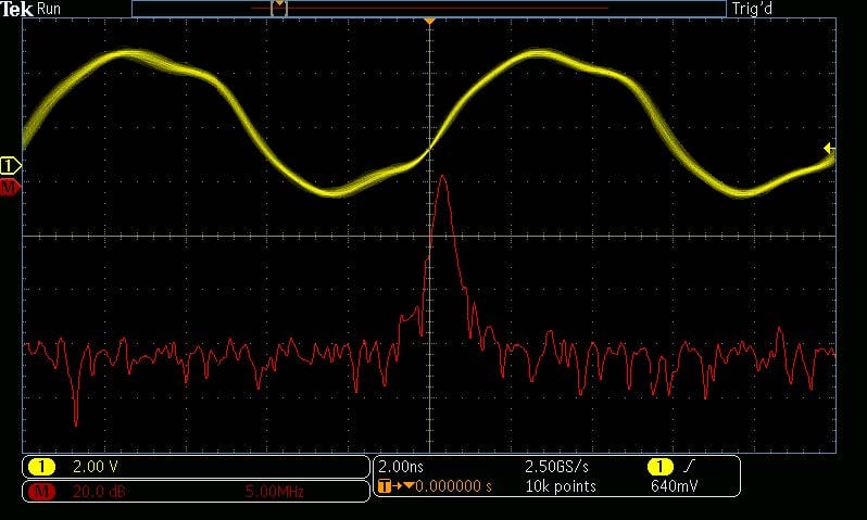 FIGURE 3. With the time domain optimized using conventional FFTs, frequency domain detail is lacking on this spread-spectrum clock signal. FIGURE 3. With the time domain optimized using conventional FFTs, frequency domain detail is lacking on this spread-spectrum clock signal. |
Spectrum View with independent controls vs. conventional FFT
Although spectrum analyzers are designed specifically for viewing signals in the frequency domain, they are not always readily available. Scopes, on the other hand, are almost always nearby in the lab so engineers tend to rely on scopes as much as possible. For this reason, oscilloscopes have included math-based FFTs (fast Fourier transforms) for decades. However, FFTs are notoriously difficult to use for two reasons.
First, for frequency domain analysis, spectrum analyzer controls like center frequency, span and resolution bandwidth (RBW) make it easy to define the spectrum of interest. In most cases, however, oscilloscope FFTs only support traditional controls such as sample rate, record length and time/div, making it difficult to get to the desired view.
Second, even if the scope offers spectrum analyzer style controls, the FFT is driven by the same acquisition system as that used for the analog time domain view. Changing the center frequency, span, or resolution bandwidth will change the scope’s horizontal scale, sample rate and record length in unanticipated and undesired ways. Once the desired frequency domain view is achieved, the time domain view of other signals is no longer usable.
When adjustments are made to horizontal scale, sample rate, or record length to again achieve the desired time domain view, the FFT view is no longer usable. For example, the next two screenshots taken from an MDO3000 illustrate the time domain and FFT views of a spread spectrum clock that moves from 97 MHz to 100 MHz. In Figure 3, the time domain view enables easy visualization of the clock, but the FFT doesn’t have adequate resolution to be useful. In Figure 4, the FFT shows the spread spectrum nature of the clock, but the time domain view is no longer helpful.
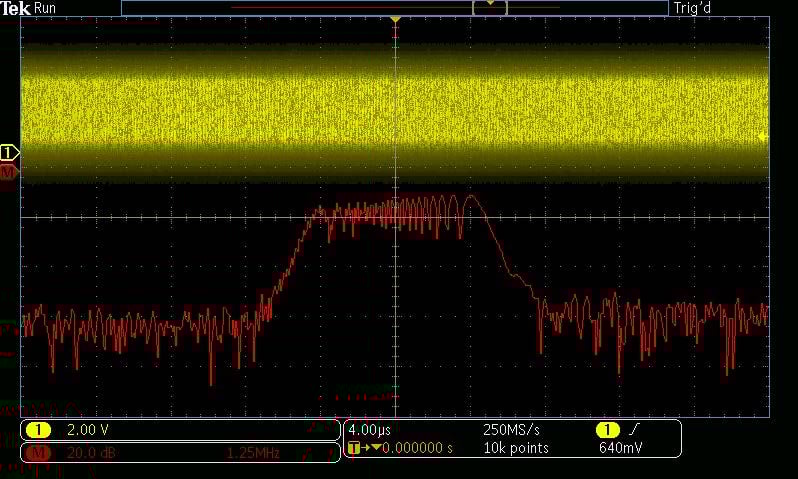
FIGURE 4. With the FFT view optimized, the time domain view of the clock signal is now not useful.
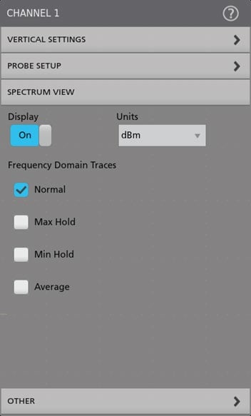
Spectrum View provides the ability to adjust the frequency domain using familiar center frequency, span and RBW controls.
And because these controls do not interact with the time domain scaling, it is possible to optimize both views independently as shown in Figure 5 below.

FIGURE 5. Looking at the same spread-spectrum clock signal as Figures 3 and 4, Spectrum View enables optimized views of both time and frequency domains at the same time.
Spectrum Time
An on-screen indicator called Spectrum Time is used to indicate where in time the spectrum shown in the Spectrum View window came from. The width of the Spectrum Time indicator is simply the Window Factor divided by the Resolution Bandwidth. (See the appendix for more on window factors.) You can move Spectrum Time throughout the acquisition to see how the frequency domain view changes over time. You can even do this on a stopped acquisition.
In Figures 6 through 9, we’ve captured the startup sequence of the spread spectrum clock discussed earlier. The Spectrum Time indicator appears very narrow in the screenshots and is highlighted by a red box to assist the reader. In this case, Spectrum Time is 1.9 (Window Factor) / 10,000 (RBW) = 190 µs wide.
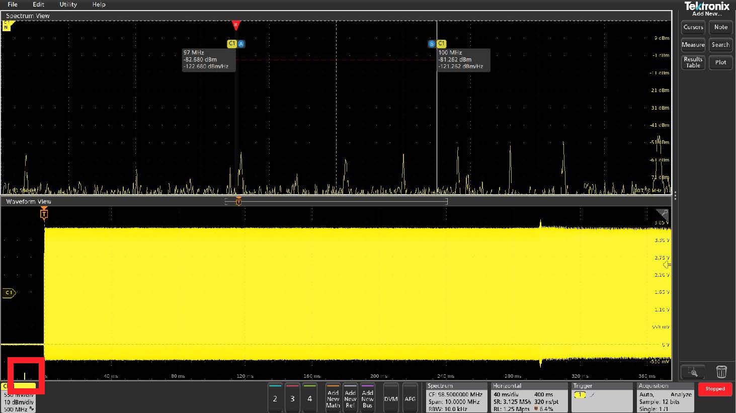
FIGURE 6. Spectrum Time (highlighted with a red box) is placed early in the acquisition, before the trigger event. As expected, there aren’t any strong signals in the frequency domain as the clock has not turned on yet.
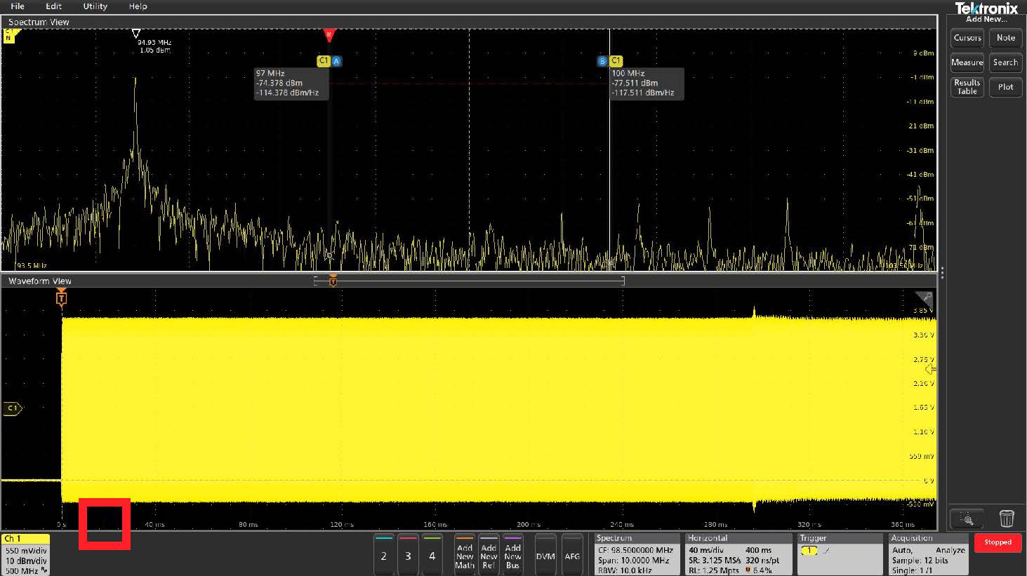
FIGURE 7. Spectrum Time placed approximately 20 ms after the clock turned on. Notice that the clock is not spread spectrum yet, it’s merely sitting at 94 MHz.
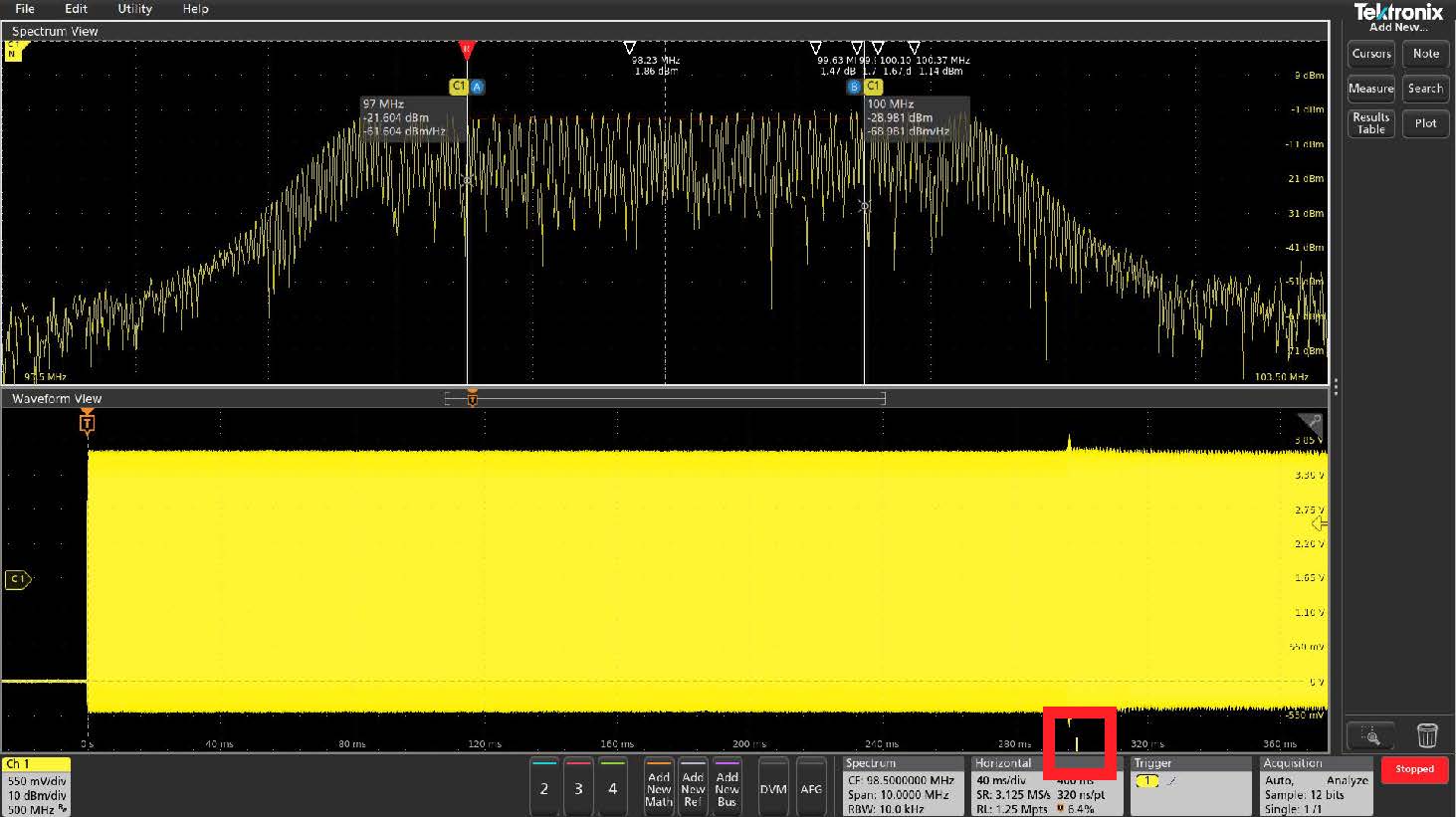
FIGURE 8. Spectrum Time placed approximately 300 ms after the clock turned on. Notice that the clock is now exhibiting spread spectrum behavior, but it’s using more of the spectrum than intended. The cursors show the expected spread spectrum width.

FIGURE 9. Spectrum Time placed approximately 324 ms after the clock turned on. Notice that the clock is now exhibiting spread spectrum behavior and is within the intended spectrum operating range.
RF vs. Time Waveforms
The underlying I&Q data that’s used to create the spectrums shown by Spectrum View can also be used to calculate RF vs. Time waveforms that show how various characteristics of the
RF waveform vary over the entire acquisition, not just where Spectrum Time is positioned. Three types of waveforms are available:
• Magnitude – The instantaneous magnitude of the spectrum vs. time
• Frequency – The instantaneous frequency of the spectrum relative to the center frequency vs. time
• Phase – The instantaneous phase of the spectrum relative to the center frequency vs. time
Each of these traces can be turned on and off independently, and all three can be displayed simultaneously. You can also trigger on these waveforms using an RF vs Time Trigger function.
These waveforms are shown in Figures 10–13 below and reveal additional information about the signal of interest. There are four time-domain waveforms shown in the Waveform View in each of the images. The top one is the analog view of the signal. Next is the RF Magnitude vs. Time waveform, then the RF Frequency vs. Time waveform, followed by the RF Phase vs. Time waveform. Finally, another RF Magnitude vs. Time waveform with the acquisition triggered off a level on the RF vs Time waveform.
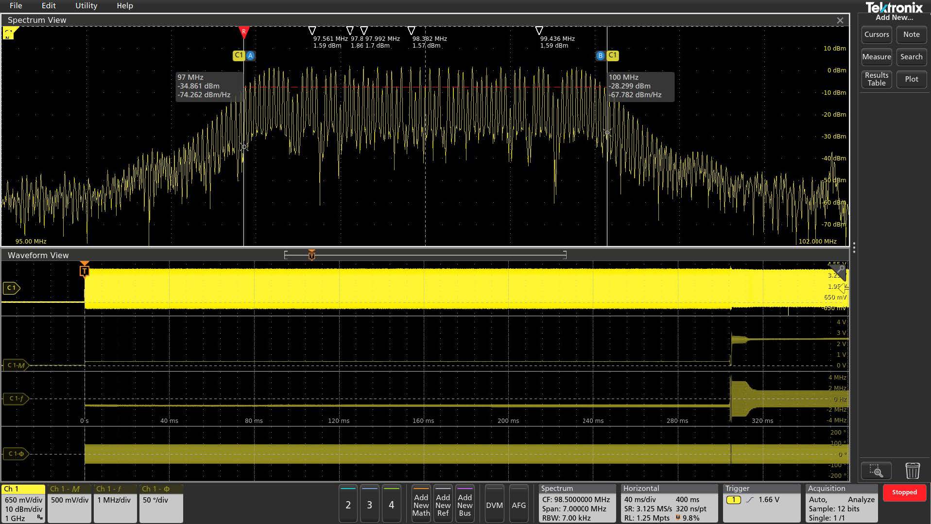
FIGURE 10. It’s very easy to see what’s going on with this spread spectrum clock by looking at the Magnitude and Frequency vs. Time waveforms. The Magnitude vs. Time trace shows the signal turning on at the trigger point at a very low level and the Frequency vs. Time trace shows the signal staying at a single frequency for the first ~300ms. At that point, we see the amplitude of the signal increase significantly and the frequency begin changing.
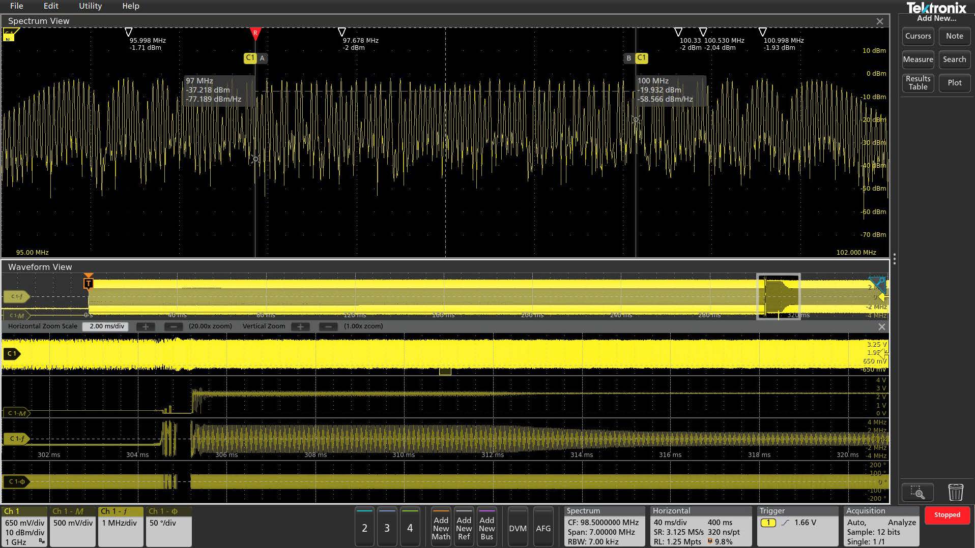
FIGURE 11. We’ve now zoomed in on the period of interest (roughly 300–320 ms after the trigger event). Notice that we can clearly see the amplitude fluctuating and the frequency changing over a broader range than it should be.
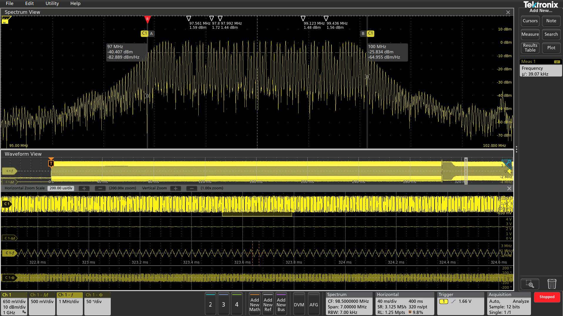
FIGURE 12. We’ve now zoomed in even further and can easily view the triangular frequency modulation in use and can confirm through the automatic measurement in the results bar that we are getting the correct modulation rate of 39.07 kHz.
FIGURE 13. To focus on the clock turn-on, we can trigger on the RF magnitude waveform by specifying a threshold and edge using an RF vs Time Trigger setting. (Note: this measurement was made with more recent firmware than Figures 10–12.)
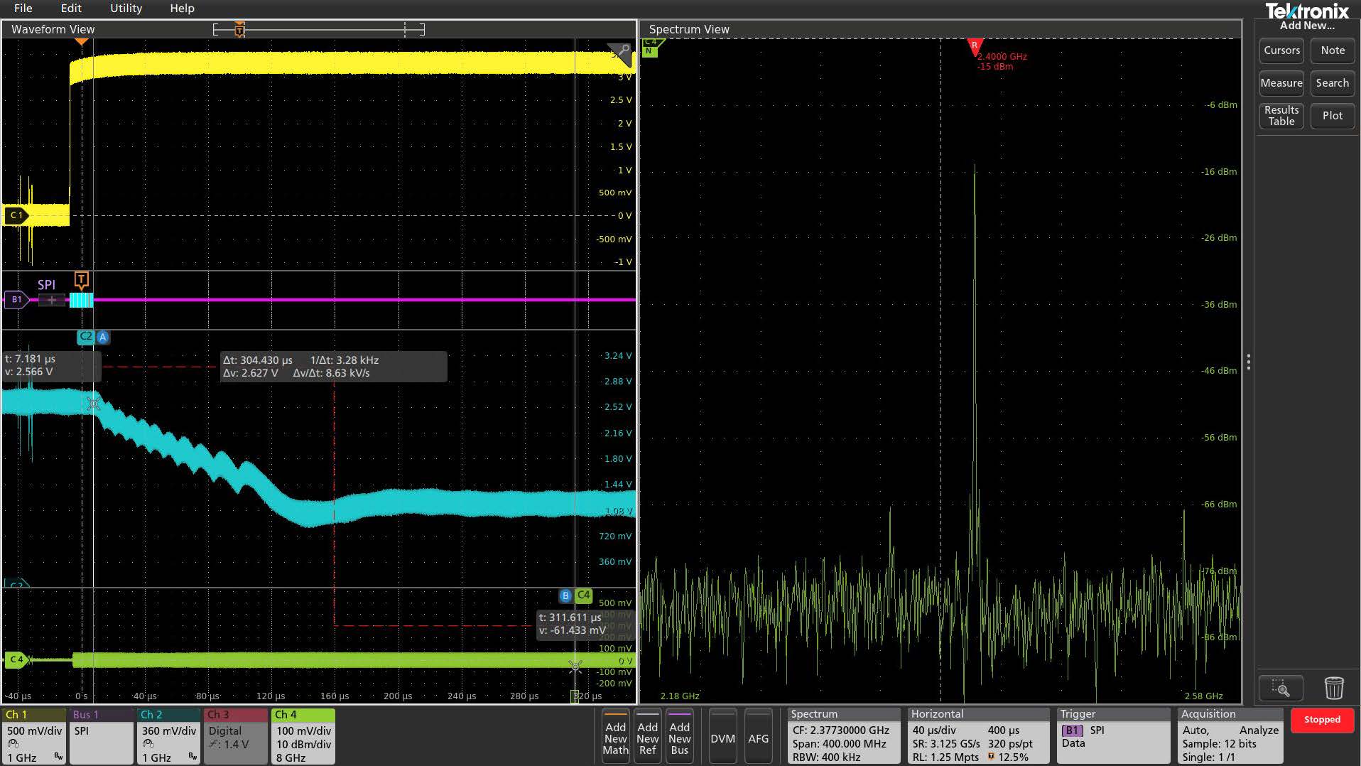
FIGURE 14. We are triggering on the SPI bus command that tells the VCO what frequency to tune to. In this case, it’s 2.4 GHz. Using Spectrum Time, we were able to scroll through the acquisition and see when the RF output stabilized at 2.4 GHz. Then, using cursors, we can measure from the trigger event to Spectrum Time’s location and see that it took 304 µs for the output to achieve the desired frequency.
Time correlation with other signals
In addition to showing how a frequency domain signal changes over time, Spectrum Time allows you to time correlate events in the frequency domain with other signals of interest in your system. In Figure 14, we’ve captured the startup of a PLL/VCO.
• Channel 1 (yellow) is the VCO enable signal
• Channel 2 (cyan) is the PLL voltage.
• Channel 3 (not shown) is configured as eight digital channels and is probing the SPI bus that controls the PLL/VCO.
• Channel 4 is the RF output.
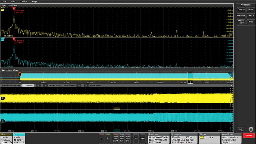 FIGURE 15. When debugging tasks demand it, multiple channels can be analyzed simultaneously. Here, two channels show the startup of a clock signal from two different points in a circuit. |
Multi-channel Analysis
For more complex troubleshooting, Spectrum View is available on multiple channels, as shown in Figure 15. Each of the two color-coded analog waveforms has a corresponding spectrum. Note that there is now a Spectrum Time indicator for each channel. By default, all Spectrum Time indicators are locked together and move together as you pan through the acquisition. This ensures you are seeing time correlated spectrums across all channels. In this example, the two channels show the startup of a clock signal from two different points in a circuit.
For very advanced troubleshooting, Spectrum Times can be unlocked and moved independently from each other. In addition the center frequency of each spectrum can be shifted independently, however all Spectrum View channels must share the same Span, Resolution Bandwidth and Window Type.
Toward More Efficient System Analysis
Efficient embedded system analysis and debugging begins and ends with insight. How can you possibly figure out why a system isn’t working as expected without precise, synchronized insight into both time and frequency domains? The answer is you can’t, and engineers have long recognized this but they have been constrained by limitations in conventional oscilloscope FFTs.
Spectrum View, enabled by next-generation ASIC technology, solves these challenges and provides a number of significant advances:
• Enables the use of familiar spectrum analysis controls (Center Frequency, Span and RBW)
• Allows optimization of both time domain and frequency domain displays independently
• Improves the update rate of the spectrum display
• Significantly improves achievable frequency resolution in the frequency domain
• Enables a signal to be viewed in both a waveform view and a spectrum view without splitting the signal path
• Enables easy investigation of how the frequency domain view changes over time and throughout an acquisition
• RF versus Time Triggers enable easy and accurate correlation of time domain events and frequency domain events
APPENDIX
A DETAILED EXAMPLE:
CONVENTIONAL FFT VS. SPECTRUM VIEW
The challenges with conventional FFTs go well beyond ease of use. To illustrate the performance tradeoffs engineers must consider, let’s say we have a tone at 900 MHz and want to view its phase noise out to 50 kHz on either side of the tone with 100 Hz resolution. Ideally, the spectral view should have the following settings:
• Center frequency: 900 MHz
• Span: 100 kHz
• RBW: 100 Hz
Conventional Oscilloscope FFT
With a traditional scope FFT, horizontal scale, sample rate and record length settings determine how the FFT works and must be considered holistically to produce the desired view.
Horizontal scale determines the total amount of time acquired. In the frequency domain, the total amount of time acquired determines your resolution. The more time you acquire, the better resolution you get in the frequency domain.
To resolve 100 Hz, we need to acquire at least (1/100 Hz) = 10 ms of time. However, in reality we need to acquire nearly double that amount of time. The beginning and end of the acquisitions introduce discontinuities (and thus error) into the resulting spectrum. To minimize these discontinuities, the acquired record is multiplied by an FFT “window”. Most FFT windows have a bell or Gaussian shape where the ends are very low and the middle is high. The resulting spectrum that is shown is primarily driven by the middle portion of the record. Each window type has a constant associated with it. For this example, using a Blackman-Harris window type with a factor of 1.90 would require that we acquire:
10 ms ×1.9=19 ms
Sample rate determines the maximum frequency in the spectrum, where Fmax = SR/2. For a 900 MHz signal, we need a sample rate of at least 1.8 GS/s. Using the analog sampling on the 5 Series as an example, we would sample at 3.125 GS/s (first available sample rate above 1.8 GS/s).
Now we can determine the record length. This is simply Time Acquired * Sample Rate. In this case, it’s:
19 ms ×3.125 GS/s = 59.375 Mpoints
Depending on the instrument, this record length may not even be available. And even if the scope has enough record length, many scopes limit the maximum length of an FFT because it is computationally intensive. For example, previous-generation Tektronix oscilloscopes have a maximum FFT length of approximately 2 Mpoints. Assuming you still want to see the 900 MHz signal (which requires the high sample rate), you’d have to acquire approximately 1/30th of the desired time resulting in 30 times worse resolution in the frequency domain than desired.
As this example illustrates, setting up a desired view requires an appreciation of the complex interactions between horizontal scale, sample rate, and record length. Moreover, the reality of finite record length forces undesirable compromise and observing high-frequency signals with good resolution in the frequency domain requires extremely long data records which are often unavailable, or expensive and time-consuming to process. Although some spectral analysis packages attempt to manage these tradeoffs, all oscilloscope FFTs to date face the limitations described above.
Spectrum View
Now let’s see how Spectrum View with the hardware digital downconversion handles the same challenge.
The total time acquired still determines the resolution in the frequency domain. We also still need to apply an FFT window and acquire data for 19 ms. In the 4, 5 and 6 Series MSOs the ADC sends digitized time domain data to a decimator to create the time domain waveform view, but it also sends the data to the digital downconverter (DDC).
As you might expect, the DDC has a profound effect on the required sample rate. The DDC shifts the center frequency of interest from 900 MHz to 0 Hz. Now the 100 kHz span goes from –50 kHz to 50 kHz. To adequately sample a 50 kHz signal, we only need a sample rate of 125 kS/s. Notice that by inserting the DDC into the acquisition process, the sample rate required becomes a function of span, not center frequency.
Record length is governed by the same relationship as before, but it is now:
19 ms ×125 kS/s = 2375 points
The data is stored as in-phase and quadrature (I&Q) samples and precise synchronization is maintained between the time domain data and the I&Q data. Remember, in the case of a conventional FFT the required record length was 59.375 Mpoints. The down-converted record only requires 2,375 points (99.996% data reduction).
Now we perform an FFT on the 2,375 point I&Q record to get the desired spectrum. This dramatic reduction in the number of data points creates several important advantages:
• Update rate is greatly improved
• Much longer timespans can be processed and thus much better frequency resolution can be achieved in spectrum analysis
• The desired frequency domain view can be captured without changing the time domain view in any way